This page walks through the diffusion example in NN.Examples.Models.Generative.Diffusion. The
model definition, training loop, sampler, and specification-level diffusion definitions are all
written in Lean.
The page follows the example from data to image artifact: where the pixels come from, how noising is represented, what the denoiser predicts, and what gets saved after a run.
Run It First
For a short runtime check, use the CUDA path with a tiny model:
lake exe -K cuda=true torchlean diffusion --cuda --dataset cifar10 --n-total 1 --steps 1 --hidden-c 1 --T 2
For a more useful local run, use CUDA if you have it. This writes a JSON loss log and a PPM image artifact so you can inspect both numbers and pixels:
python3 scripts/datasets/download_example_data.py --cifar10

lake exe -K cuda=true torchlean diffusion --cuda --fast-kernels \
  --dataset cifar10 --n-total 800 --steps 50 --hidden-c 8 \
  --log data/model_zoo/diffusion_trainlog.json \
  --sample-ppm data/model_zoo/diffusion_sample.ppm
The command is small enough to run locally, but it still exercises the full path: data conversion, typed tensors, runtime model, sampler, and saved artifacts.
Data: Where Images Come From
TorchLean does not decode JPEG/PNG inside Lean. Image decoding and resizing happen before Lean; the
Lean side receives fixed-layout .npy tensors and checks their shapes.
Once the arrays exist, the Lean side loads NCHW tensors, checks the shape and class range, and
batches them.
The two dataset modes in NN.Examples.Models.Generative.Diffusion are:
- CIFAR-10 as
(N, 3, 32, 32)arrays. - ImageNet-style folders converted to
(N, 3, 64, 64)arrays (Imagenette, Tiny-ImageNet, or any folder with class subdirectories).
Inside the example, the loader path is straightforward:
- Build a labeled source over
.npyfiles. - Load it into a dataset.
- Create a shuffled batch loader.
- Map pixel values from
[0, 1]into the diffusion range[-1, 1].
That last step is a single line in the example code:
def toDiffusionRange (x01 : Tensor Float (x0Shape c h w)) :
    Tensor Float (x0Shape c h w) :=
  Spec.Tensor.mapSpec (fun x => 2.0 * x - 1.0) x01
The Spec Layer: What We Mean By “Diffusion”
TorchLean keeps diffusion vocabulary in NN.Spec.Generative.Diffusion.*. This is the layer that
lets “training code”, “sampler code”, and “theorems” talk about the same objects.
The DDPM picture is simple enough to state before the formulas: add noise to an image at timestep
t, train a model to predict the noise that was added, then run reverse steps that use the model’s
noise prediction to move back toward a clean image. TorchLean gives each component a named
definition so the runtime command and theorem-facing modules use the same vocabulary.
At the center is an interface for an epsilon-prediction denoiser:
structure EpsModel (α : Type) (s : Shape) [Context α] where
  eps : Tensor α s → α → Tensor α s
The forward noising process is the standard DDPM formula, but written as a total tensor definition:
def qSample (sched : VPSchedule α T)
    (x0 : Tensor α s) (t : Fin (T + 1)) (eps : Tensor α s) :
    Tensor α s :=
  let αbar : α := sched.alphaBar t
  let c0 : α := sqrtNonneg αbar
  let c1 : α := sqrtNonneg (1 - αbar)
  Tensor.scaleSpec x0 c0 + Tensor.scaleSpec eps c1
The training objective is also named at the spec level:
def epsPredLoss (sched : VPSchedule α T) (model : EpsModel α s)
    (x0 : Tensor α s) (t : Fin (T + 1)) (eps : Tensor α s) : α :=
  let x_t := qSample sched x0 t eps
  let tScalar : α := VPSchedule.timeOfIndex (α := α) (T := T) t
  let epsHat := model.eps x_t tScalar
  Spec.mseSpec epsHat eps
Then the surrounding spec modules define:
- a discrete VP schedule
VPSchedulewithβ_t,α_t = 1-β_t, and cumulative productsᾱ_t; -
two reverse samplers:
- DDPM: a stochastic reverse step with explicit per-step noise inputs,
- DDIM (η = 0): a deterministic reverse step that reuses the same denoiser but drops the noise.
There are also “hooks” that let diffusion samplers plug into the generic dynamical-system API. For
example, the DDIM spec exposes ddimStepSystem and proves the step definition by rfl so other
theory can rewrite it safely.
The Runtime Layer: The Model That Runs
The runnable diffusion command does not work directly with EpsModel. It instantiates a concrete
neural network and then uses the public data API to build training samples.
Two choices matter in the example:
- The epsilon predictor is a residual CNN that preserves resolution
(
epsResidualConvNet). The training, sampling, and visualization path stays easy to run on a local checkout. - Time is fed to the model as an extra channel: the input has
(data channels + 1)channels, where the last channel is the normalized timestep broadcast across spatial positions.
That “append time as a channel” trick is defined once in the API:
def appendTimeChannel {batch c h w : Nat}
    (x : Spec.Tensor Float (NN.Tensor.Shape.NCHW batch c h w)) (tNorm : Float) :
    Spec.Tensor Float (NN.Tensor.Shape.NCHW batch (c + 1) h w) := ...
The model is a same-resolution residual CNN sized to run as an example. This is a compressed excerpt of the real definition; the source file expands each convolution with the exact tensor shapes and seeded initializers:
def epsResidualConvNet (cfg : EpsConvNetConfig) :
    nn.M (nn.Sequential (epsConvNetInShape cfg) (epsConvNetOutShape cfg)) :=
  nn.sequential![
    conv3x3SameImages,
    nn.relu,
    residualBlock,
    nn.relu,
    residualBlock,
    nn.relu,
    conv3x3SameImages
  ]
The important bit for the tutorial is the contract: input is noisy NCHW image plus time channel,
output is predicted noise with the original image shape.
Training: What Gets Optimized
Training is classic DDPM-style ε-prediction. Each step:
- pick a real image batch
x0, - pick a timestep
t, - sample noise
ε, - build a supervised pair
(appendTimeChannel x_t tNorm, ε), - take an optimizer step on MSE.
TorchLean makes the supervised pair explicit as a SupervisedSample value. The operation that
constructs x_t from x0 and ε is NN.API.diffusion.noisedSampleFromEps; it is the runtime
version of the same formula used by qSample in the spec layer.
The excerpt below leaves out the local definitions of sqrtAb, sqrtOneMinusAb, and tNorm, but
keeps the actual tensor transformation:
def noisedSampleFromEps
    (alphaBars : Array Float) (T : Nat)
    (x0 eps : Tensor Float (NN.Tensor.Shape.NCHW batch c h w)) (step : Nat) :
    SupervisedSample Float
      (NN.Tensor.Shape.NCHW batch (c + 1) h w)
      (NN.Tensor.Shape.NCHW batch c h w) :=
  let x_t :=
    Spec.Tensor.scaleSpec x0 sqrtAb +
    Spec.Tensor.scaleSpec eps sqrtOneMinusAb
  Sample.mk (appendTimeChannel x_t tNorm) eps
Sampling: DDIM Replay In Lean
The example uses deterministic DDIM because it is easy to audit and stable at small scale.
The reverse update used by the runnable example is NN.API.diffusion.ddimPrev. It does the usual
“predict x0, clip, remix” step:
- estimate
x0_hatfromx_tandε̂, - clamp it to
[-1, 1], - recombine it using the previous schedule coefficients.
The implementation is just that recipe. Here is the compact form, with the schedule coefficients shown by name:
def ddimPrev
    (abPrev ab : Float)
    (x_t epsHat : Tensor Float (NN.Tensor.Shape.NCHW batch c h w)) :
    Tensor Float (NN.Tensor.Shape.NCHW batch c h w) :=
  let x0Hat :=
    Spec.Tensor.scaleSpec
      (Spec.Tensor.subSpec x_t (Spec.Tensor.scaleSpec epsHat sqrtOneMinusAb))
      (1.0 / (if sqrtAb > 1e-12 then sqrtAb else 1e-12))
  let x0Clipped := Spec.Tensor.clampSpec x0Hat (-1.0) 1.0
  Spec.Tensor.scaleSpec x0Clipped sqrtAbPrev +
    Spec.Tensor.scaleSpec epsHat sqrtOneMinusAbPrev
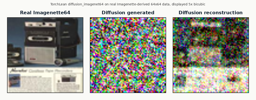
This is also where the example produces the “three pictures” view:
- a reference image (real
x0), - a noisy image at a chosen timestep,
- a reconstruction from DDIM reverse steps starting at that timestep.
What To Look At After A Run
Diffusion is one of the easiest places to fool yourself, so the example pushes you toward artifacts: images on disk and a JSON curve log. That gives you something concrete to compare across CPU/CUDA, fast-kernel switches, schedule tweaks, or model width changes.
For interactive inspection, open NN.Examples.Models.Generative.Diffusion in VS Code with the Lean
Infoview enabled. The widgets can display tensor summaries, graph and shape views, and saved JSON
logs next to the source.
Source entry points: